
distribution of conductance-based synaptic noise
Neural Comput. 17: 2301-2315, 2005

Abstract
Synaptically generated subthreshold membrane potential (Vm) fluctuations can be characterized within the framework of stochastic calculus. It is possible to obtain analytic expressions for the steady-state Vm distribution, even in the case of conductance-based synaptic currents. However, as we show here, the analytic expressions obtained may substantially deviate from numerical solutions if the stochastic membrane equations are solved exclusively based on expectation values of differentials of the stochastic variables, hence neglecting the spectral properties of the underlying stochastic processes. We suggest a simple solution that corrects these deviations, leading to extended analytic expressions of the Vm distribution valid for a parameter regime that covers several orders of magnitude around physiologically realistic values. These extended expressions should enable finer characterization of the stochasticity of synaptic currents by analyzing experimentally recorded Vm distributions and may be applicable to other classes of stochastic processes as well.
Complementary Information and Material
1. NEURON demo
NEURON demo program to simulate the fluctuating conductance model, calculate its steady-state Vm distribution, and compare it to the extended analytic expression obtained in the paper: ZIP (4 kByte)
To run the demo, unzip this file, compile the mod file mechanism and execute the file demo.hoc.
2. Examples of fitting distributions for extreme parameter regimes
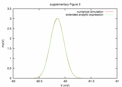
Below we present a number of supplementary figures which compare the Vm distributions obtained from numerical simulations and using the extended analytic expression for extreme parameter sets. Please note that the chosen parameters (e.g. very small or very large time constants) approach the limit of computational methods on currently available generic computer systems (Dell precision workstation, Pentium 4 with 3 GHz with 3 GigaByte total memory running under the Linux operating system). To assess the numerical errors (see Section 3 below) we performed in all cases various simulations for given model parameters but different integration time steps, length of simulated neural activity and random number seed.
Please note that the model parameters chosen here go beyond physiologically realistic values by several orders of magnitude. They were chosen to evaluate the limits of the extended analytic expression for the Vm distribution!
Notations:| T | simulated neural activity | |
| dt | integration time step for numerical simulation | |
| a | membrane area (in square microns, μm2) | |
| G | total membrane conductance | |
| GL | leak conductance | |
| C | membrane capacity | |
| τm | passive membrane time constant | |
| τ0 | total membrane time constant | |
| ge0, gi0 | mean of excitatory and inhibitory conductances | |
| σe, σi | standard deviations of excitatory and inhibitory conductances | |
| τe, τi | excitatory and inhibitory conductances noise time constants |
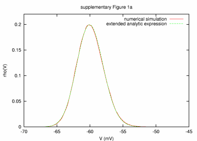 |
Model of a small cell (38 μm2) with small membrane time constant (0.005 ms) PARAMETERS: T = 100 s, dt = 0.0005 ms, a = 38 μm2, C = 0.00038 nF, G = 75.017176 nS, GL = 0.017176 nS, τm = 22.1 ms, τ0 = 0.005 ms, ge0 = 15 nS, gi0 = 60 nS, σe = 2 nS, σi = 6 nS, τe = 2.7 ms, τi = 10.5 ms. |
|
| REMARKS: In this model parameter set, a small effective membrane time constant of about 0.005 ms was obtained by decreasing the area of the membrane to 38 μm2. Although the analytic expression captures very well the Vm distribution obtained by numerical simulation, we observed a slight mismatch, in particular on the depolarised tail of the Vm distribution. To investigate the source of this mismatch, we ran simulations with integration time steps of 0.00025 ms (shown, T = 50 s), 0.0005 ms (T = 100 s), 0.001 ms (T = 100 s) and 0.005 ms (T = 100 s). The amplitude of the mismatch decreased systematically for smaller dt, suggesting that the source of error is linked to the numerical integration procedure utilised in our simulations. | ||
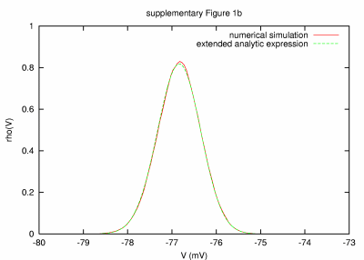 |
Model with high leak and small membrane time constant (0.005 ms) PARAMETERS: T = 100 s, dt = 0.0005 ms, a = 10000 μm2, C = 0.1 nF, G = 23728.4 nS, GL = 19978.4 nS, τm = 0.005 ms, τ0 = 0.00421 ms, ge0 = 750 nS, gi0 = 3000 nS, σe = 150 nS, σi = 600 nS, τe = 2.7 ms, τi = 10.5 ms. |
|
| REMARKS: In this model parameter set, a small leak and effective membrane time constant of about 0.005 ms were obtained by increasing the leak and synaptic conductances. The match between analytic expression and numerical simulation result is excellent. As for the case shown in supplementary Fig. 1a, simulations with different integration time steps were performed to assess to which extend the small deviations (in particular at the peak of the distribution) can be assigned to the numerical integration procedure. Also here we observed a slow but systematic decrease in the deviation for decreasing integration time step. | ||
 |
Model of a large cell with large membrane time constant (5 sec) PARAMETERS: T = 10000 s, dt = 0.1 ms, a = 100000 μm2, C = 1.0 nF, G = 0.1952 nS, GL = 0.0452 nS, τm = 22124 ms, τ0 = 5123 ms, ge0 = 3.0e-5 nS, gi0 = 12.0e-5 nS, σe = 1.5e-5 nS, σi = 6.0e-5 nS, τe = 2.7, τi = 10.5 |
|
| REMARKS: A large membrane time constant of 5 s in the presence of synaptic activity was obtained by a large membrane area and very small leak and synaptic conductances (passive time constant is 22 s). Various integration time steps and length of simulated activity were considered, and the deviation between numerical and analytic result decreased for longer T and smaller dt. However, some deviations are linked to the fact that the standard deviation of the synaptic noise used was only half the mean conductances, leading to a 2.3% chance of encountering negative conductances, which cannot be captured in this approach (see Section 3 below). | ||
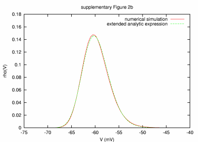 |
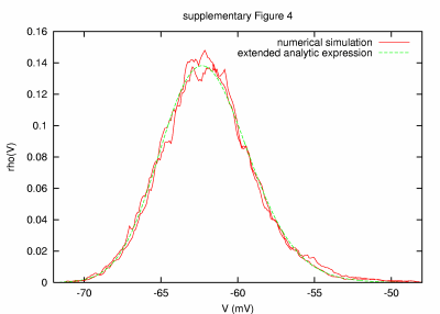
Model with low leak and long membrane time constant (50 sec) PARAMETERS: T = 10000 s, dt = 0.1 ms, a = 20,000 μm2, C = 0.2 nF, G = 75.003996 nS, GL = 0.00399568 nS, τm = 50054 ms, τ0 = 2.67 ms, ge0 = 15 nS, gi0 = 60 nS, σe = 3 nS, σi = 12 nS, τe = 2.7 ms, τi = 10.5 ms. |
|
| REMARKS: In this model parameter set, a very large passive membrane time constant of 50 s was chosen by reducing the leak membrane conductance. This large time constant made it necessary to consider long simulated activity. However, due to principal limitations of our computational resources, the latter prohibited the use of very small integration time steps. In turn, a slight mismatch seen between the numerical result and analytic expression was observed, which decreased systematically when smaller integration time steps were considered. We performed simulations with dt = 0.2 ms (T = 20,000 s), dt = 0.5 ms (T = 50,000 s) and dt = 1 ms (T = 100,000 s). | ||
 |
Model with small noise time constants (0.005 ms) PARAMETERS: T = 100 s, dt = 0.0005 ms, a = 20000 μm2, C = 0.2 nF, G = 84.04 nS, GL = 9.04 nS, τm = 22.12 ms, τ0 = 2.38 ms, ge0 = 15 nS, gi0 = 60 nS, σe = 3 nS, σi = 12 nS, τe = 0.005 ms, τi = 0.005 ms. |
|
| REMARKS: In this simulation, very small time constants for both excitatory and inhibitory synaptic conductances were used. The length of the integration time step was a crucial source of the observable mismatch between numerical result and analytic expression (investigated dt and T values were the same as for supplementary Fig. 1a). | ||
 |
Model with large noise time constants (50 sec) PARAMETERS: T = 20000 s, dt = 0.1 ms, a = 20000 μm2, C = 0.2 nF, G = 84.04 nS, GL = 9.04 nS, τm = 22.12 ms, τ0 = 2.38 ms, ge0 = 15 nS, gi0 = 60 nS, σe = 3 nS, σi = 12 nS, τe = 50000 ms, τi = 50000 ms. |
|
| REMARKS: Here, very long time constants of 50 s for both excitatory and inhibitory noise were considered. The match between the numerical result and the analytic expression is very good, given the fact that the smallest time constant in the system (τ0 about 2 ms) sets a stringent limit for the integration time step, whereas the long noise time constants require the simulation of very long neural activity. Simulations performed with various dt and T indicate that the main source of the observed mismatch is due to the limitation in the length of simulated neural activity (in the case shown in the figure, T was only 400 times larger than the noise time constants). The shown figure contains the result of two numerical simulations (red) obtained by using different random seeds while all other simulation and model parameters were the same. | ||
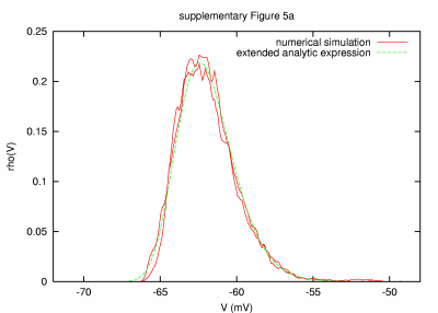 |
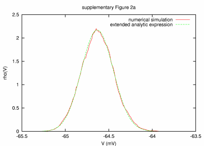
Model with disparity in time constants, fast for excitation (0.01 ms) and slow for inhibition (1 sec) PARAMETERS: T = 200 s, dt = 0.001 ms, a = 20000 μm2, C = 0.2 nF, G = 84.04 nS, GL = 9.04 nS, τm = 22.12 ms, τ0 = 2.38 ms, ge0 = 15 nS, gi0 = 60 nS, σe = 3 nS, σi = 12 nS, τe = 0.01 ms, τi = 1000 ms. |
|
| REMARKS: In this parameter set, a mixture of very small and large noise time constants are considered. Please note that the time constants for excitation and inhibition differ by 5 orders of magnitude, which puts very strong constraints on the numerical simulation. The integration time step must be small enough to capture the effects of the fastest process (we show the result for an only 10 times smaller dt compared to te), whereas the simulated activity must be long enough to ensure significant statistics to capture the effects of the slowest process (we choose T = 200 s, which is only 200 times longer than ti). Changing dt and T, the amplitude of the observed mismatch can be modified, suggesting limits in the used numerical integration method. Here, longer simulated activity decreases systematically the observed mismatch, indicating that for this parameter set inhibition plays the most significant role. The shown figure contains the result of two numerical simulations (red) obtained by using different random seeds while all other simulation and model parameters were the same. | ||
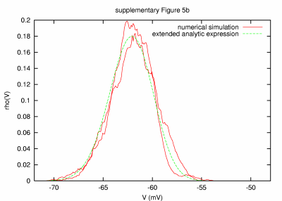 |
Model with disparity in time constants, slow for excitation (1 sec) and fast for inhibition (0.01 ms) PARAMETERS: T = 200 s, dt = 0.001 ms, a = 20000 μm2, C = 0.2 nF, G = 84.04 nS, GL = 9.04 nS, τm = 22.12 ms, τ0 = 2.38 ms, ge0 = 15 nS, gi0 = 60 nS, σe = 3 nS, σi = 12 nS, τe = 1000 ms, τi = 0.01 ms. |
|
| REMARKS: Idem preceding figure, but excitation and inhibition noise time constants were switched. | ||
3. Limits of the extended analytic expression
Theoretical limits:
To date, we are aware of two principal limitations of the proposed extended analytic expression for the full conductance-based model, which are linked to the theoretical approach along which it was obtained. These are:
-
Incorporation of negative conductances.
Due to the Gaussian nature of the distribution of the conductance noise processes, the presence of unphysical negative conductances cannot be accounted for in the analytic approach. This will lead to a mismatch between numerical simulations and analytic solution in situations where the probability of negative conductances can no longer be neglected, e.g. for a value of the noise standard deviation close to its mean. For example, already a noise standard deviation which is half the value for the mean, at average 2.3% of the conductances are expected to be negative. The sudden change in the sign of the driving force due to negative conductances has an impact on the dynamics of the system which is not accounted for in the analytic approach. A possible solution could be to make use of qualitatively different stochastic processes for conductances, e.g. described by Gamma-distributions.
-
Crossing of conductance reversal potentials.
Eventual changes in the sign of the driving force due to crossing of the conductance reversal potentials, which practically will play a role only for inhibition, lead to a different dynamic behaviour of the numerical model which, due to the exclusive use of expectation values and averages, can not be captured in the analytic approach. The expected deviations are most visible at membrane potentials close to the reversal potentials and/or large values of the involved conductances. Possible solutions under investigation include the use of different numerical integration methods as well as the use of different boundary conditions for the distribution.
Numerical limits:
Because the validity of the analytic result can only be probed by comparison with numerical simulations, an assessment of the limits of the computational approach as well as the resulting numerical error must be made.
-
Integration time step vs. length of simulated activity.
The most crucial limitations (and source of error) in the numerical approach are the length of the integration time step and the simulated activity. Whereas the integration time step should, ideally, be much smaller than the smallest time constant of the system, only a long simulated neural activity will provide enough statistics to ensure a valid membrane potential distribution. Although, in principle, there are no limits for these quantities, an upper limit of file size and simulation time sets stringent constraints. To reduce this error, we approached the limits of the available computer system by statistically considering neural activity amounting to 200 Million datapoints. To assess the impact of the integration time step, various simulations with various integration time steps were performed in all cases. In general, the deviation between numerical and analytic result decreased systematically the smaller the chosen integration time step and the larger the simulated activity.
-
Procedure for solving numerically differential equations.
No known method for numerical integration is error-free. In general, the errors expected are larger for fixed-time step integration methods compared to variable time-step methods. Unfortunately, due to the involvement of noise, we are bound to use fixed-time step methods. Here we observed that for extreme parameter sets (such as very large conductance values, sets with a non-neglectible probability for negative conductances, sets leading to neural activity close to the reversal potential) the numerical integration was unstable, yielding a major source of deviations with the analytic result. This behaviour was particularly pronounced for sudden changes of the sign of the driving force (e.g. by crossing the reversal potential or the occurrence of negative conductances).
-
Correctness of the random number generator.
A less expected but significant source of error was linked to the generation of the noise using pseudo-random numbers. Although the method used by NEURON is the best available trade-off between speed of random-number generation and "quality" (true randomness) of the random numbers, we observed non-neglectible deviations from the desired values. Deviations of 0.5% (considering the average over 1 Million generated random numbers) from the desired values in both mean and variance of generated random numbers were not rare. Although small, deviations of this size especially for the standard deviation do have an impact on neural dynamics, and the resulting statistical characterisation of the membrane potential distribution, in particular for extreme parameter sets, as the ones shown above. Moreover, small deviations of the spectral properties of the generated noise processes from the Lorentzian (expected for OU stochastic processes) were observed.